In the Physics Module you define the radiative properties of gas and dust components.

This section covers how to access and use the interface functionality. For a more detailed account of the underlying physical and numerical procedures and assumptions, please refer to the Theory section of the manual or to the PDF document "Radiative Transfer in Shape".

In general, we have tried to keep the physical calculations in line with the general philosophy of Shape, i.e. keep it simple and fast, but good enough to capture the most important phenomenology to allow qualitative and first order quantitative analysis.

Units: Note that contrary to most of the astrophysics literature, in Shape we use Standard International (SI) units, i.e. MKS units based on meter, kilogram and seconds. For example, astronomers used to thinking in terms of particles per ccm should multiply all the densities by 1e6 before they put them into the density modifier. Unit conversions can be done easily on a number of websites nowadays, e.g. at UnitConversion.

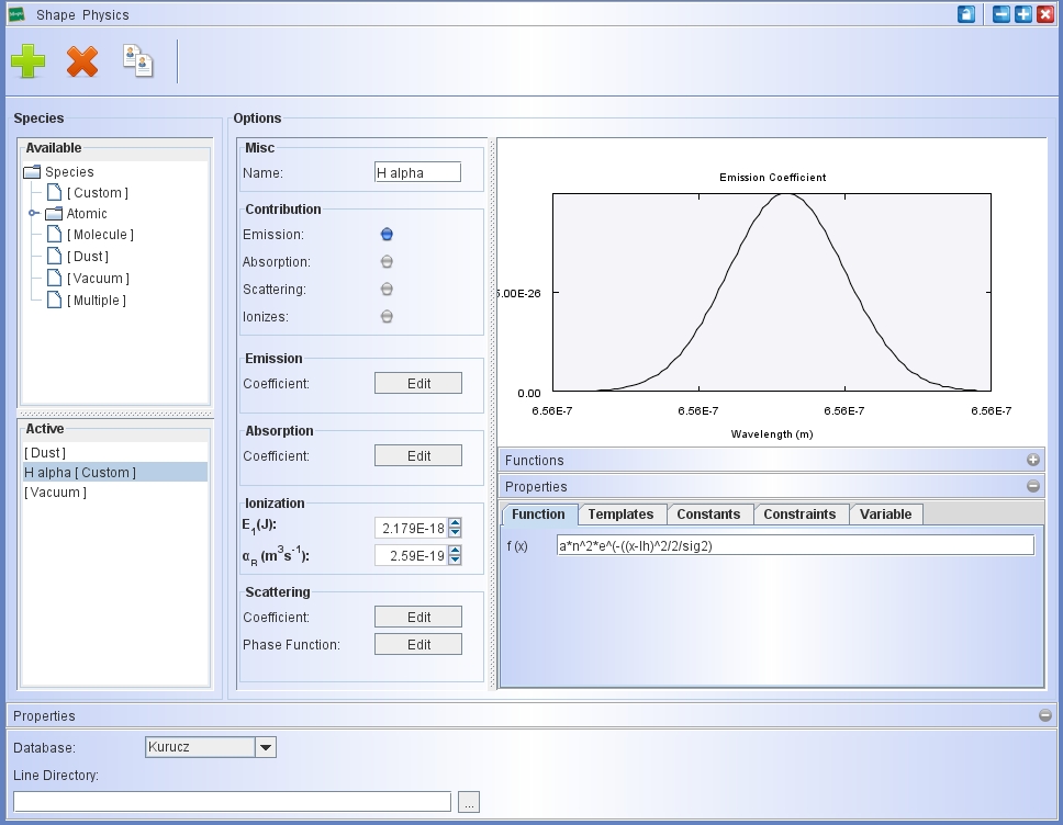
The basic procedure is to define material species for which you specify their radiative properties. These are then assigned to a geometric object in the Species panel of the 3D Module. You first select a basic species from the Species list and add it to the Active list by drag & drop or by clicking on the green "+"-button at the top. Now select the species in the Active window. In the Options window on the right you can now set the detailed properties of this species.

You define the emissivity, absorption and scattering coefficients as a function of wavelength. First activate one of these coefficients in the Contribution area (there may be more than one active) and the Edit their wavelength dependence. See the Graph section of the manual for a more detailed description of the Graph functionality.

In the graph, when using an analytical function, the variables n and t give direct access to the density (by number) and temperature fields, respectively, as provided by the corresponding modifiers in the 3D Module.

Currently, there are five different basic species available: Custom, Dust, Atomic, Vacuum, and Multiple.
The Molecule option is currently only a placeholder for future use.

In the Custom species you set all properties manually according to your needs that might not be available in other species that have some property presets.

Atomic is actually an extensive list of atomic species from which you can choose. Those have access to two extensive spectral line databases (Kurucz and Chianti) which provide atomic coefficients for line intensity calculations.

The Dust species allows to set dust properties for emission and scattering calculations. Currently, for each species you have only a single grain size. A more complex distribution can be approximated by using several species of different grain sizes and densities.

Note that a limitation of current dust and atomic calculations in Shape is that the temperature is set either manually as spatial distribution or as a function of some other parameter, but they are not calculated as part of the radiation transfer.

The Vacuum species is to set regions associated with a geometric shape as empty. In the Particle System list of the 3D Module any object that is located below a given vacuum object will be empty in this region. Objects located above the vacuum object in the list will be unaffected. This is an extremely powerful help when complex density structures have to be set up.

Custom		Top
The Custom allows you to manually set Emission, Absorption and Scattering as a function of wavelength.
If you make complex objects with several species, it is easier to keep track of the individual species when you give them proper Name in the corresponding text field at the top of the Options panel. Then you choose how this species contributes to the radiation transfer, i.e. by Emission, Absorption, Scattering and/or Ionization. You can choose more than one of these. Then define the details of the individual contributions in their corresponding graphs as a function of wavelength (click on the corresponding Edit button).

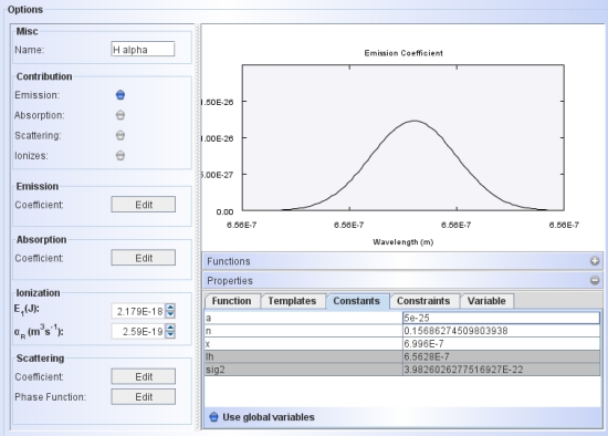An Ionization potential E_1(J) can be assigned in units of Joule. Similarly, the recombination coefficient α_R can be set in SI (mks) units.

There is also an option to set the Scattering coefficient and its Phase Function (see the Dust species for more on that topic).

Dust	Demo project: dust_demo_shape2010.shp	Top
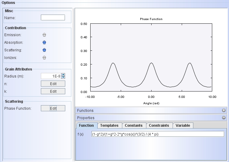
The dust species has the options to contribute by Emission, Absorption and Scattering.
The grain attributes include their radius (single radius, not a distribution), the index of refraction with the real part n and the complex part k. k controls the absorption. Both, n and k can be set as a function of wavelength, by editing the corresponding graph (click on the Edit button).

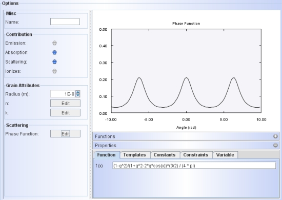The Scattering currently is single scattering. Dust scattering calculations have the option to include a scattering phase function. To see and edit the function click on the Edit button to the right of the label Phase Function. The preset is the Henyey-Greenstein function. The single parameter g of this function can be changed in the constants tab of the graph. The user can change this function.

For scattering calculations remember that you need at least one Emitter object in the 3D Module. The properties of the Emitter can be set after you select Emitters from the Object Type drop-down menu at the top-right of the 3D Module.

Demoproject:
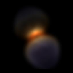
The following images are outputs from the dust demo project that you can download: dust_demo_shape2010.shp

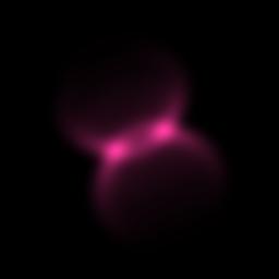
The objects is a simple bipolar dust structure with a central star (Emitter object) at a blackbody temperature of 20000 K. The emission is from scattered light only. Moderate forwards scattering is included with g=0.3.
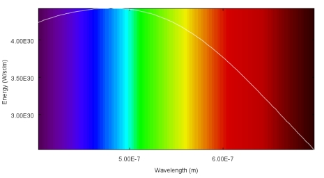
On the left is the rendered image (make sure to activate the rainbow image mode) and on the left is the total continuum spectrum (shown in the Plot Module) .

The atomic species allows to calculate the emission properties based on the atomic transition coeffcients and the physical conditions like density and temperature in the object.

IMPORTANT NOTE:
Usage of atomic species for the calculation of emission and absorption requires detailed knowledge of the underlying physics. We recommend the application of this option only for users that are experienced in this area. Testing of the atomic calculations in Shape has been limited so far. It is advised you solve your own test problems comparing the results either with analytical calculations or computations with other established programs. We would actually appreciate to receive notice of any results of such comparisons. We can then include those in the documentation of Shape and apply pertinent improvements or corrections.

You have the choice from two large databases for the atomic coefficients: Kurucz and Chianti.
To use this feature download the line databases for Shape here. Unpack the compressed archive in a suitable directory and direct the Line Directory to the appropriate subdirectory (Kurucz or Chianti).

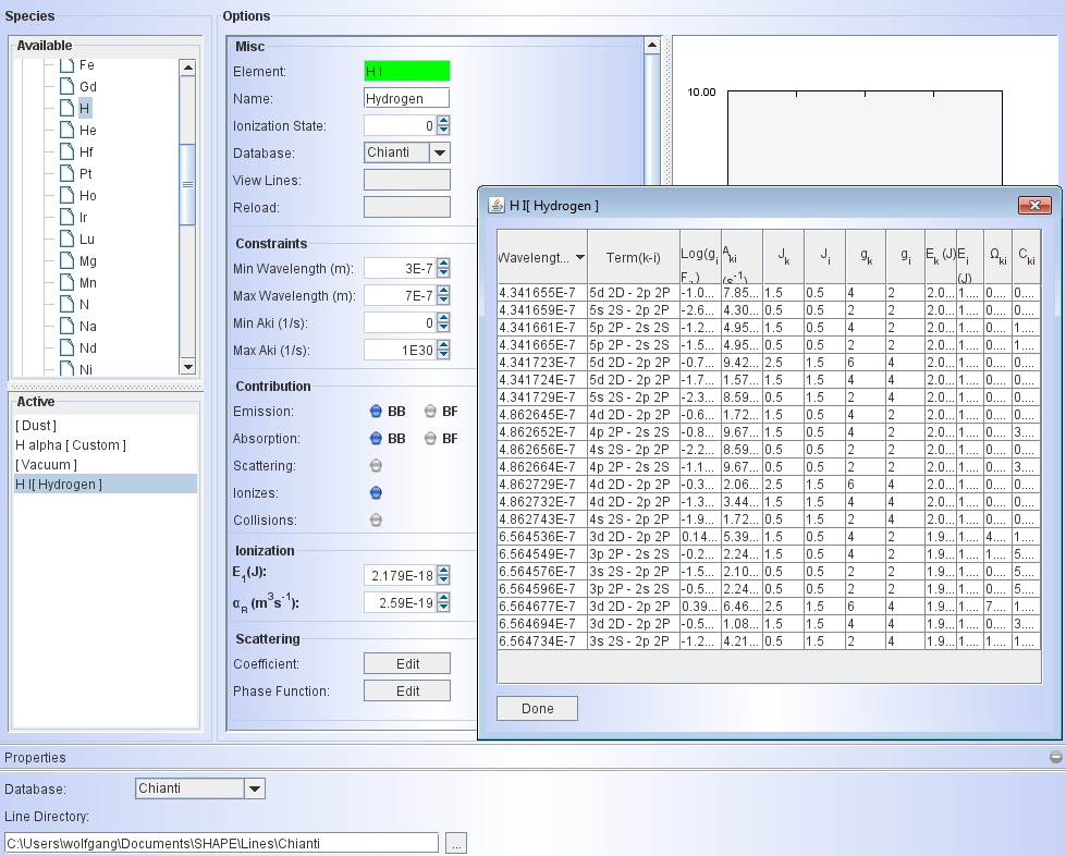
To apply one or the other database select the Database at the bottom of the Species Panel. Then point the Line Directory to the corresponding directory on your harddisk. If you have not done so before, first download the database here and unpack the zip-file in a suitable location. Now select the Ionization State of the species in the Misc panel of the Options. For hydrogen the ionization state has to be set to "0", because discrete lines only occur for neutral hydrogen. Processes that involve free electrons, i.e. Bound-Free (BF), take the next higher ionization state into account automatically.

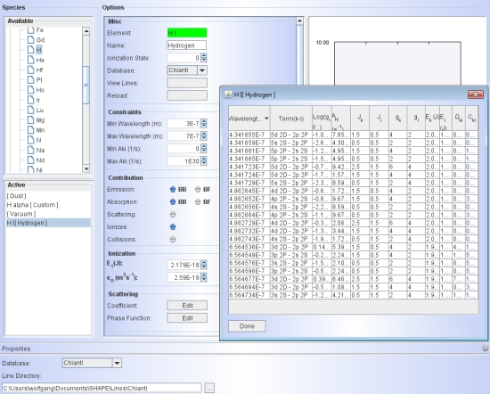Now select the Database for this particular species in the Misc panel from the corresponding drop-down menu. Click on the Reload button to read the lines. If the background of the Element label changes from red to green, then you successfully read the lines. If it is still red, one or more of the settings are incorrect. This could be the directory for the lines, the ionization state is not available for this atom or something similar.

To see a listing of the lines and their atomic properties click on the View Lines button. It shows a table of the atomic properties in the database. If you want to see only the lines in a certain wavelength interval, you can set Constraints for a minimum and maximum wavelength, as well as for the minimum and maximum Einstein coefficients (e.g. to select for allowed or forbidden lines).

The Contributions area allows you to select from various radiative process to be included in the calculations. The label B stands for Bound and F for Free. Note that not all processes are available for all the atoms, except for hydrogen. Please contact the authors for details.

The Ionization potential that appears by default is that of hydrogen. This is true also for other species. So, make sure to find the ionization potential for other species from external sources, e.g. at ChemGlobe. Conversions of electron-volt (eV) energy units to Joule can be easily done at the following site: UnitConversion. Recombination coefficients for many species can be obtained, e.g., from Verner and Ferland (1995).

The Scattering has the option of a scattering phase function. To see and edit the function click on the Edit button to the right of the label Phase Function. The preset is the Henyey-Greenstein function. The single parameter g of this function can be changed in the constants tab of the graph. The user can change this function.

Demoprojects:
The following images are outputs from the atomic species demo projects that you can download: atomic_demo_shape2010.shp

Remember that for this and all projects that use the atomic species you need to download the lines database and point the Lines directory to the appropriate directory in your filesystem.

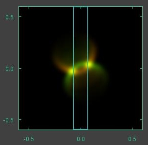
The objects is a simple bipolar hydrogen recombination emission structure.
On the left is the rendered image (make sure to activate the rainbow image mode) and on the left is the total spectrum (shown in the PV diagram display ). The discrete line spectrum shows the Balmer series and has been displayed with a square root brightness table. Note red/pink total color of the image that is dominated by the Hα line

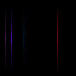
The second demo project includes only the Hα and uses a very narrow wavelength range. A narrow slit is used to produce a position-velocity diagram of this line. The color coding is according to the Doppler-shift. Note that in this this project only a single spectral line was included from the line list (click on the View Lines button).

atomic_demo_pv_shape2010.shp

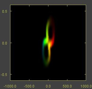
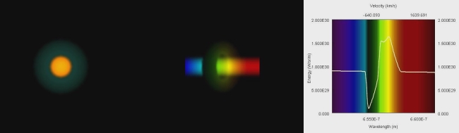
P-Cygni profiles are important diagnostic tool for stellar wind and circumstellar medium research. Here is a demo project for such a profile. The geometric setup are to simple spheres, one for the star and one for the wind or expanding shell. The star is opaque and has a flat continuum emission. For the wind a single spectral line (Hα) has been set up with the Physics Module including emission and absorption. The temperature is constant at 15000 K (set with the Temperature modifier in the 3D Module). The velocity field increases linearly with distance. The project has an animation setup changing the thickness of the expanding wind shell such that it is initially thin, increasing thick until the inner edge reaches the stellar surface. The spatially resolved position-velocity gives interesting insight in how the P-Cygni profile works (center in the image below), especially in the animation. This project makes use of the Plot Module for the visualization of the P-Cygni profile.

To use the demo project for the P-Cygni profile (see below) make sure to have downloaded, installed and loaded the Kurucz spectral line database (see above).

Download the animation and the demo project (Shape version 2010).