| |
In Shape graphs are used to display functions. The functions are either analytical or set interactively by adding control points to a piecewise linear curve. The control points of an interactive curve can also be loaded from an external ascii file.
In modifiers the graphs are usually applied to set and display spatial variation of a quantity, while in the Physics Module it commonly is as a function of wavelength.
The functionality of the graphs varies slighty depending on the particular purpose. We show the properties of the graph with the most features. Other graphs derive from this one, but might not have features that are not needed for its particular application.
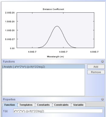
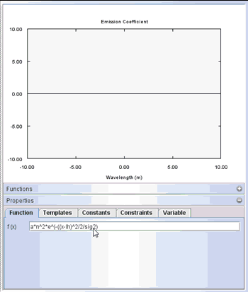
The image of the graph on the right is taken from the Physics Module and is the gaussian emissivity curve of the Hα line.
The graph is divided in three different sections from top to bottom: the function display, a function stack and the properties panel.
The function display shows a line of how the function f(x) changes as a function of the independent variable (by default x).
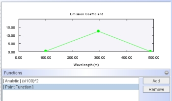
The function stack allows you to combine several functions that may be of different type. They are multiplied with each other. This is useful in cases where it is more practical to define several short functions and combine them later, instead of writing a big formula. It also allows to combine, perturb or taper analytical functions with interactive functions. In the modifiers of the 3D Module, such a combination can be achieved by combining several modifiers of the same type. In the Physics Module the function stack makes it possible to achieve a similar combination.
At the bottom is a list of tabs to set a variety of function properties. |
Click on the image to see a higher resolution version.
|
|
| Function display |
|
Every function has a useful range in x and f(x) where the interesting action happens. Therefore it is important to set these ranges accordingly. Otherwise nothing might be visible in the graph.
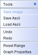
The setting of the display can be accessed via the right-click menu (with the mouse on the function display). From this menu select Graph Properties.
Note that the right-click menu for the interactive point graph (left figure) and the analytic graph (right) are different. In addition to those in the analytic menu, the point menu has special functions to manipulate the control points of the curve.
Zooming and Panning: To interactively zoom in or out use the mouse wheel. Click and drag with the middle mouse-button pressed to pan around the graph. You can restrict the zooming to one direction by simultaneously pressing the x- or y-keys. |
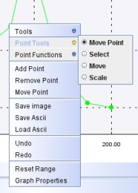
Right-click menu of point graph. |
Right-click menu of analytic graph |
| |
|
|
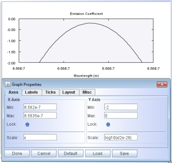
In the Graph Properties dialog you can customize the function graph. To set the ranges for the axes open the Axes tab. Type the appropriate minimum and maximum values in the corresponding text fields. As usual, make sure to confirm the values by pressing the keyboard Enter. If the Lock button is activated, then the range might not change when entering the values. In that case deactivate the Lock and confirm the values again.
The scaling for the axes may be changed by entering a formula in the Scale text boxes. They can be set to any mathematical expression. Make sure to use x for the name of the variable on both axes! In the example on the right, the y-axis has been set to a logarithmic scale. The function is the same as the gaussian in the top figure.
|
| |
|
In the Label tab the graph can be customized in terms of colors, lines and font. You can set a Graph Title. Try different settings to find the most suitable. The visibility of the defaults might be inappropriate for publications or presentations. An image of the graph can be saved using the Save Image command that becomes availbale when you right-click on the graph.
An important setting is the Format String, which allows you to set the precision of the numbers.
Similar menus are available to set the properties of tick marks, layout (margin sizes) and miscellaneous parameters of the panel. |
|
| |
|
|
This gif animation shows how to customize a graph such that a predefined gaussian spectral line shape is shown in an appropriate form.
First, the right-click menu is used to open the graph properties panel.
Then the ranges are adjusted using the information of the line center and height.
Finally, some adjustments are made to the look of the graph. |
|
| Function stack |
|
|
The function stack is available only in the Physics Module. It produces a similar functionality as combining several modifiers in the 3D Module. Currently, they are combined by multiplication.
Stacking several functions can be useful, e.g., when you have an analytical background function and wish to perturb this smooth function by a custom interactive point function; or you might have a diverging analytical function in a certain region and want to taper it off with an point function.
To add a new function to the stack, first click on the Add button, select the type of function you wish to use and the edit the properties (see next section). |
|
| Function properties |
|
The function properties are divided into several sections and are accessed via the tabs at the bottom of the graph panel.
The interactive point functions have only one option, i.e. a button to load an ascii file with data that will be used to set the function.
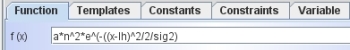
An analytic function can be typed in the Function tab. Most common mathematical operators can be used with there usual symbols. The example on the left shows a gaussian line profile, where all basic operators are used (+-*/), but also the exponent (^). |
|
There are several reserved names. e is the Euler number, pi is ...Pi, n is the number density taken from the density modifier, ST is temperature. The math interpreter does not distinguish lower and upper case letters, e.g. T or t are interpretated the same.
|
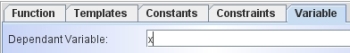
By default the independent variable is always x. You can change the name of the independent variable in the Variable tab. Any non-reserved string is valid.
|
|
|
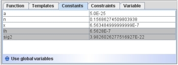
If you include letters or words that are not reserved (like those mentioned before and others like trigonometric functions) these strings are interpreted as constants. The appear in the Constants tab. Here you can assign numerical values to them. If you have set global variables in the Math Module then you can use them here by activating the Use global variables button at them bottom of the Constants tab. These variables are marked with a different background color.
|
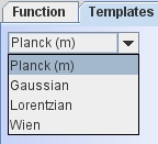
Some commonly used functions can be quickly inserted into the Functions tab by selecting them from the Templates tab. These can then be quickly taylored to the specific form needed in a particular problem.
|
|
|
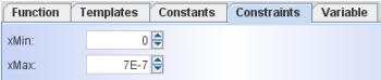
Sometimes the range over which one wishes to apply a functions is limited, e.g. for diverging functions like 1/x or similar. You can set Constraints, i.e. a range of the independent variable, outside of which the function is set to zero. |
|