 ) for each spectral
feature is obtained by measuring the decrease
in flux due to line absorption from the
continuum that is expected when interpolating between two
adjacent bands, defined here as the blue continuum
band [BCB] and the red continuum band [RCB].
The equivalent width W is defined as
:
) for each spectral
feature is obtained by measuring the decrease
in flux due to line absorption from the
continuum that is expected when interpolating between two
adjacent bands, defined here as the blue continuum
band [BCB] and the red continuum band [RCB].
The equivalent width W is defined as
: FB, BCB, and RCB) of the feature
band and continuum bands, respectively, and
FB, BCB, and RCB) of the feature
band and continuum bands, respectively, and  FB is the width of
the FB. Equivalent widths or "indices" measured
by this procedure are largely insensitive to reddening
as long as the wavelength coverage of each band
is relatively small. Indices constructed in this way
should also be quite independent of the S/N as
long as the sidebands are chosen to be next to
the measured feature and are wide enough to obtain
a good flux estimate. Thus, judicious selection of
the width of each band relies on a compromise
between minimizing reddening effects and maximizing the
S/N.
FB is the width of
the FB. Equivalent widths or "indices" measured
by this procedure are largely insensitive to reddening
as long as the wavelength coverage of each band
is relatively small. Indices constructed in this way
should also be quite independent of the S/N as
long as the sidebands are chosen to be next to
the measured feature and are wide enough to obtain
a good flux estimate. Thus, judicious selection of
the width of each band relies on a compromise
between minimizing reddening effects and maximizing the
S/N.| # |
NAME |
Central Wavelength (A) |
Spectral type range |
| 1 |
CaII(K) |
3933 |
A0-G0 |
| 2 |
FeI+ScI |
4047 |
F5-K1 |
| 3 |
MnI |
4032 |
B5-G9 |
| 4 |
HeI |
4026 |
O8-B3; B3-A0 |
| 5 |
CN |
4175 |
O8-A5; F5-G9 |
| 6 |
HeI |
4144 |
O8-B3; B3-A1; F5-K3 |
| 7 |
TiII+FeII |
4203 |
F2-K4 |
| 8 |
CaI | 4226 |
F2-K3 |
| 9 |
TiII, FeII, CrII | 4176 | O8-A7 |
| 10 |
FeI |
4271 | F2-K5 |
| 11 |
CH(Gband)
|
4305 | F2-G2 |
| 12 |
HeI+FeI |
4387 |
O8-B3; B3-A1; F2-K4 |
| 13 |
MnI+FeI
|
4458 | F2-K4 |
| 14 |
HeI |
4387 |
O8-B2; B2-A1; A7-K1 |
| 15 |
MnII |
4481 |
B5-A1 |
| 16 |
FeI |
4490 |
B5-A1 |
| 17 |
FeI |
4532 |
A0-G5 |
| 18 |
FeI |
4592 |
B5-K4 |
| 19 |
FeI+ScII |
4669 |
O8-B3; B2-G2 |
| 20 |
FeI |
4787 |
A5-K3 |
| 21 |
HeI+FeI |
4922 |
O8-B2; B2-A1; A7-K4; K5-M6 |
| 22 |
HeI+FeI+TiI |
5016 |
A0-K5 |
| 23 |
FeI |
5079 |
A0-K3; K5-M6 |
| 24 |
FeII+MgI |
5173 |
A0-G0 |
| 25 |
FeI+CaI |
5270 |
A0-K0 |
| 26 |
FeI |
5329 |
F2-K5 |
| 27 |
FeI |
5404 |
O8-B2-F5-K5 |
| 28 |
HeI |
5878 |
O8-A0; G9-M0 |
| 29 |
CaI |
5589 |
A0-K3; M0-M6 |
| 30 |
MgI |
5711 |
A5-K5;K5-M6 |
| 31 |
NaI |
5890 |
F2-G2; G9-K7 |
| 32 |
MnI |
6015 |
F2-K5 |
| 33 |
CaI |
6162 |
F5-K3; K0-K7 |
| 34 |
HeI |
6678 |
B2-A0 |
| 35 |
HeI |
7066 |
O8-A1;M0-M6 |
| 36 |
Halpha |
6565 |
O8-A1;A0-K7 |
| 37 |
Hbeta |
4861 |
O8-A1;A1-G0 |
| 38 |
Hgamma |
4349 |
O8-A1;A1-K6 |
| 39 |
TiO |
6185 |
M0-M6 |
| 40 |
TiO |
6720 |
K5-M6 |
| 41 |
CaH |
6975 |
K2-M6 |
| 42 |
CaH |
6385 |
K1-M6 |
| 43 |
CaH |
6830 |
K2M6 |
| 44 |
Hdelta |
4102 |
O8-A1;A1-F9 |
| # |
Name |
Central wavelength |
Spectral type rages |
| 1 |
Ca I |
4226 |
G0-M0 |
| 2 |
Gband |
4290 |
F5-K5 |
| 3 |
Fe I |
4370 |
F5-K4 |
| 4 |
Fe I |
4458 |
A5-K5 |
| 5 |
Mg I |
5170 |
F0-K4 |
| 6 |
Ca I |
5277 |
F5-K5 |
| 7 |
Fe I |
5329 |
F5-K5 |
| 8 |
Fe I |
5406 |
G0-K4 |
| 9 |
Ca I |
5590 |
F5-K5 |
| 10 |
Fe I |
5709 |
G0-K5 |
| 11 |
Ca I |
6165 |
G0-K5 |
| # |
Name | Central wavelength | Spectral type rages |
| 1 |
TiO1 |
4775 |
K3-M6 |
| 2 |
TiO2 | 4975 |
K3-M6 |
| 3 |
TiO3 | 5225 |
K0-M6 |
| 4 |
TiO4 | 5475 |
K4-M6 |
| 5 |
TiO5 | 5600 |
K3-M6 |
| 6 |
TiO6 | 5950 |
K6-M6 |
| 7 |
TiO7 | 6255 |
K2-M6 |
| 8 |
TiO8 | 6800 |
K3-M7;M7-M9.5 |
| 9 |
TiO9 | 7100 |
K5-M7;M7-M9.5 |
| 10 |
TiO10 | 7150 |
K5-M7;M7-M9.5 |
| 11 |
VO1 |
7460 |
M5-M9;M9-L0 |
| 12 |
VO2 | 7940 |
M0-M9;M9-L0 |
| 13 |
VO3 | 7840 |
M0-M8;M8-M9.5 |
| 14 |
VO4 | 8500 |
M0-M9;M9-L0 |
| 15 |
VO5 | 8675 |
M0-M9;M9-L0 |
| 16 |
VO6 | 8880 |
M0-M9;M9-L0 |
 Figure 2: initial box
 FIGURE 3: main box
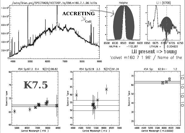
 Figure 4: Important
lines. In this example you can see the infrared Ca II triplet,
the infrared O I (7773, 8446) doublette and the line He I (6676)
in emission
supporting that this object is a strong accretor.
Figure 4: Important
lines. In this example you can see the infrared Ca II triplet,
the infrared O I (7773, 8446) doublette and the line He I (6676)
in emission
supporting that this object is a strong accretor.  Figure 5: Manual
Classification. This option requires some experience in
spectral classification. If you are not sure about using this option
select
the option NO_CLASSIFIED (last option second column in main box)
Figure 5: Manual
Classification. This option requires some experience in
spectral classification. If you are not sure about using this option
select
the option NO_CLASSIFIED (last option second column in main box) Figure 6: Chossing
the scheme for interactive classification.
Figure 6: Chossing
the scheme for interactive classification.
 Figure 8: Equivalent
width of Halpha. The green line shows the position at 6563A. The
purple line is the gaussian line fitted to the feature.
Figure 8: Equivalent
width of Halpha. The green line shows the position at 6563A. The
purple line is the gaussian line fitted to the feature. Figure 9: Comment box.