Hydrodynamics
Lessons in this section are a basic introduction to the hydrodynamics module. The preprint of the research paper that will describe the numerical procedure of the hydrodynamics and a first application will soon be available here. In this section we describe the basic setup and the test runs that we have performed so far. The supernova project file can be downloaded here. It is used as the demo project for this series of tutorials. This page also presents standard tests of the hydrodynamic code for comparison with analytical predictions.
Note that the Hydro Module in Shape runs 3D simulations on a regular cubic grid. No 1D or 2D simulation with symmetry assumption are done. This is due to the overall concept of how Shape works internally. This puts some restrictions on the simulations that can be done in terms of hardware, resolution and time it takes to run them. For publication grade simulations we recommend a 64 bit system with over 10 GB of RAM (which have to be made available to Shape in the file "Shape_v5.0.vmoptions" that is located in the installation directory). Since the code is parallelized using threading it takes advantage of multiple CPU cores. Hence the more cores you have, the faster the simulation runs.
Return to Learning Center.
1- Setup of a hydro scene in the 3D module |
Video playlist on YouTube Click on "Playlist" at the bottom of the video for access to individual lessons. For best viewing you might want to switch to full screen video and use a HD setting for the video quality (buttons in the lower right corner of the video). |
||||||||
|
2- The hydrodynamics module |
|||||||||
|
3- Rendering hydrodynamic objects |
|||||||||
4- Hydro graphs |
|||||||||
Modules and features involved |
|||||||||
|
Graph |
Math |
Physics |
Filters |
|||||
Hydro code numerical scheme and test results
Hydrodynamic simulation codes are based numerical procedures for which there are many options, each of which has advantages and disadvantages compared to others. This initial version of the code in Shape is designed to provide a basic tool to simulate the structure and evolution of nebulae that involve shocks produced by winds or explosions with cooling. This was to be achieved with a minimal computational effort, to make it interactively usable on desktop computers and workstations, rather than clusters or supercomputers. Still, the code is fully threaded, which means that it can take advantage of multi-core architectures, with corresponding speed-ups
The numerical scheme is a second order upwind shock-capturing Godunov method including a van Leer flux--vector splitting (van Leer, 1982). For more details see the research paper on the code (Steffen et al., 2013, MNRAS, submitted). Cooling is treated as a parameterized three-segment linear (in log-log space of temperature and energy loss) approximation above 10^4 K. Below 10^4 K there is no cooling at this time, the peak is at log(T/K)=5.5 and the free-free starts at log(T/K)=7.5.
In this section we present a few tests that illustrate the degree of accuracy of the implementation.
Supernova Test Here we compare the expansion of a supernova explosion with cooling to the theoretical curves expansion for the two regimes of adiabatic (Sedov-Taylor) phase and the momentum driven phase after cooling of the expanding shell. This also tests the working of the cooling procedure, which provide approximately the correct cooling time for such a strong explosion. Parameters: The initial environment has constant particle density of n=10^6 m^(-3), i.e. rho_env = 0.6 m_H n, where m_H is the mass of the hydrogen atom. This value for the density includes the assumption that it is ionized and takes into account the contribution by helium. The computational domain has a physical size of 50 parsec (1.542x10^18 meters) and a 3D grid of 200^3 cells. The supernova has been initialized in a spherical region of radius r0 = 3 parsec (9.257x10^16 meters), corresponding to 12 cells. The density was set to be rho_sn = rho_env + 3/4 pi r0^3 / m_sun, where m_sun is the solar mass. The energy of the supernova was set to 10^51 erg, which corresponds to 10^44 Joule (Shape uses SI units). Both, the environment and the SN gas are assumed stationary at the initial state of the computation. |
|
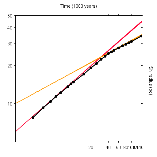 |
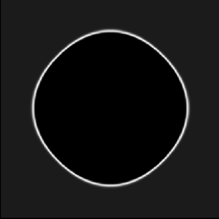
The radius of the dense supernova shell is shown as a function of time (left), together with the theoretical curves for the Sedov-Taylor phase (red) and the momentum driven phase after cooling of the shell (orange). Below is shown a cut through the density distribution in the central x-y plane is shown for the final time at 150 kyears. |
 |
|
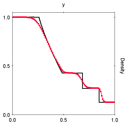
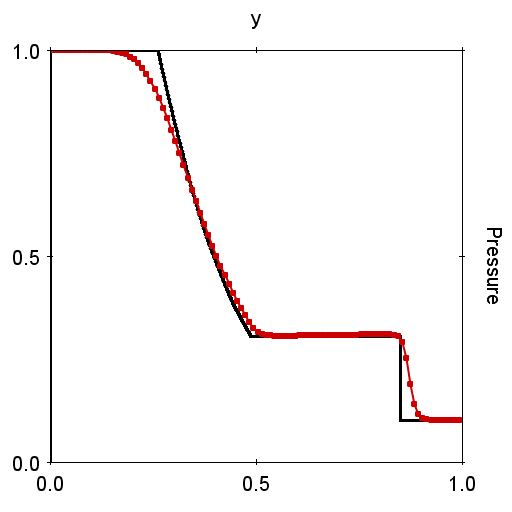
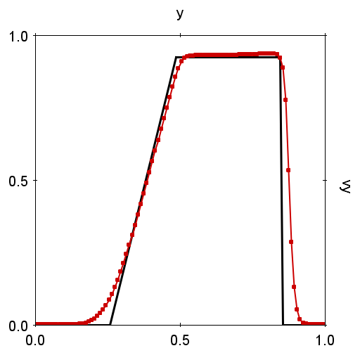
For a theoretical description of this test see the following page on Wikipedia and the references therein. The test was performed using fixed 3D grid with 200^3 cell. Using the Filter Module we then extracted a column of 1 cell width from the center of the domain along the direction of propagation of the shock. We present the density, pressure and velocity (red lines with dots) compared with the theoretical curves as plotted in the Graph Module. |
|
 |
|
 |
|
 |
|